Examples#

A copy‑paste, minimal example#
Copy paste the code in this section to just get the pipeline working quickly.
We do a cursory analysis of the Lotka‑Volterra, predator‑prey differential‑equation model. This is often used as a toy example for global‑sensitivity‑analysis tools; see e.g. the following links:
– <https://cran.r-project.org/web/packages/ODEsensitivity/vignettes/ – https://diffeq.sciml.ai/v6.9/analysis/global_sensitivity/
– https://strimas.com/post/lotka-volterra/. Because it’s really simplesimple.Note that one of the model features we analyse is non‑differentiable. Mathematically that would be a problem, but computationally everything works fine – we’ll explain why later.
Lotka‑Volterra model of predator‑prey interactions#
The dynamics for the system are
$$ \begin{aligned} \frac{d\text{🐁}}{dt} &= p_1\text{🐁} - p_2 \text{🦉} \text{🐁} \\ \frac{d\text{🦉}}{dt} &= -p_3\text{🦉} + p_4 \text{🐁} \text{🦉} \end{aligned} $$
- \(p_1\) and \(p_2\) are the birth and death rates of the mice.
- \(p_3\) and \(p_4\) are the birth and death rates of the owls.
… and here is a time‑course of their populations when p = [1.5, 1.0, 3.0, 1.0].
We call these values the nominal parameters.
Nominal system (i.e. simulated with nominal parameter values)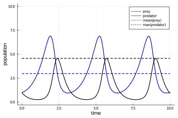
We will follow two features of interest:
- mean population of the mice over time,
- max population of the owls over time.
The model‑feature vector for the nominal system is \([2.98,,4.57]\).
Our cost function on model behaviour is the mean‑square deviation these nominal features.
By the way
In your ecology class you may have heard of \(r/K\) selection. This is (criticised) theory that there are two extremal strategies that species trade off between:
- r‑strategists (e.g. rabbits): high birth and death rates, low investment per individual.
- K‑strategists (e.g. humans): low birth and death rates, high investment per individual.
We will use this terminology in our description of the MD curves.
- By running the code at the bottom of the page twice, setting
which_dir = 1andwhich_dir = 2respectively, we obtain two MD curves (see below).
Minimally disruptive curve 1#
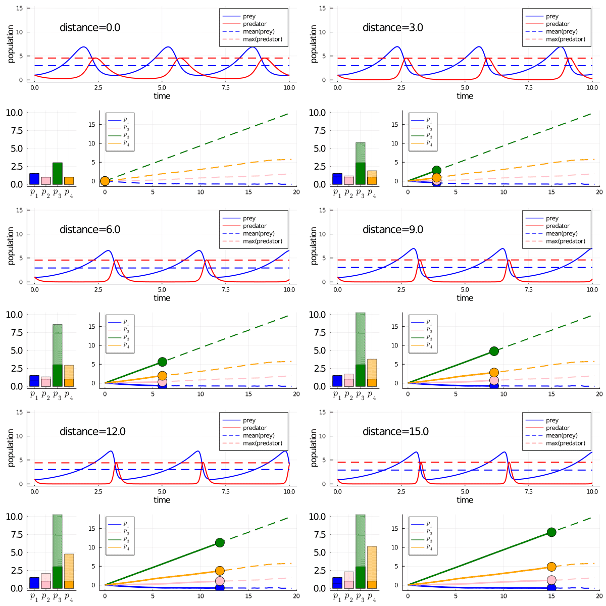
- As we move along the curve, predators move towards an \(r\)-strategy and prey move towards a \(K\)-strategy.
- We can also move in the opposite direction (prey to \(r\) strategy, predator to \(K\)). To avoid figure clutter, run the pasted code yourself to see this!
Minimally disruptive curve 2#
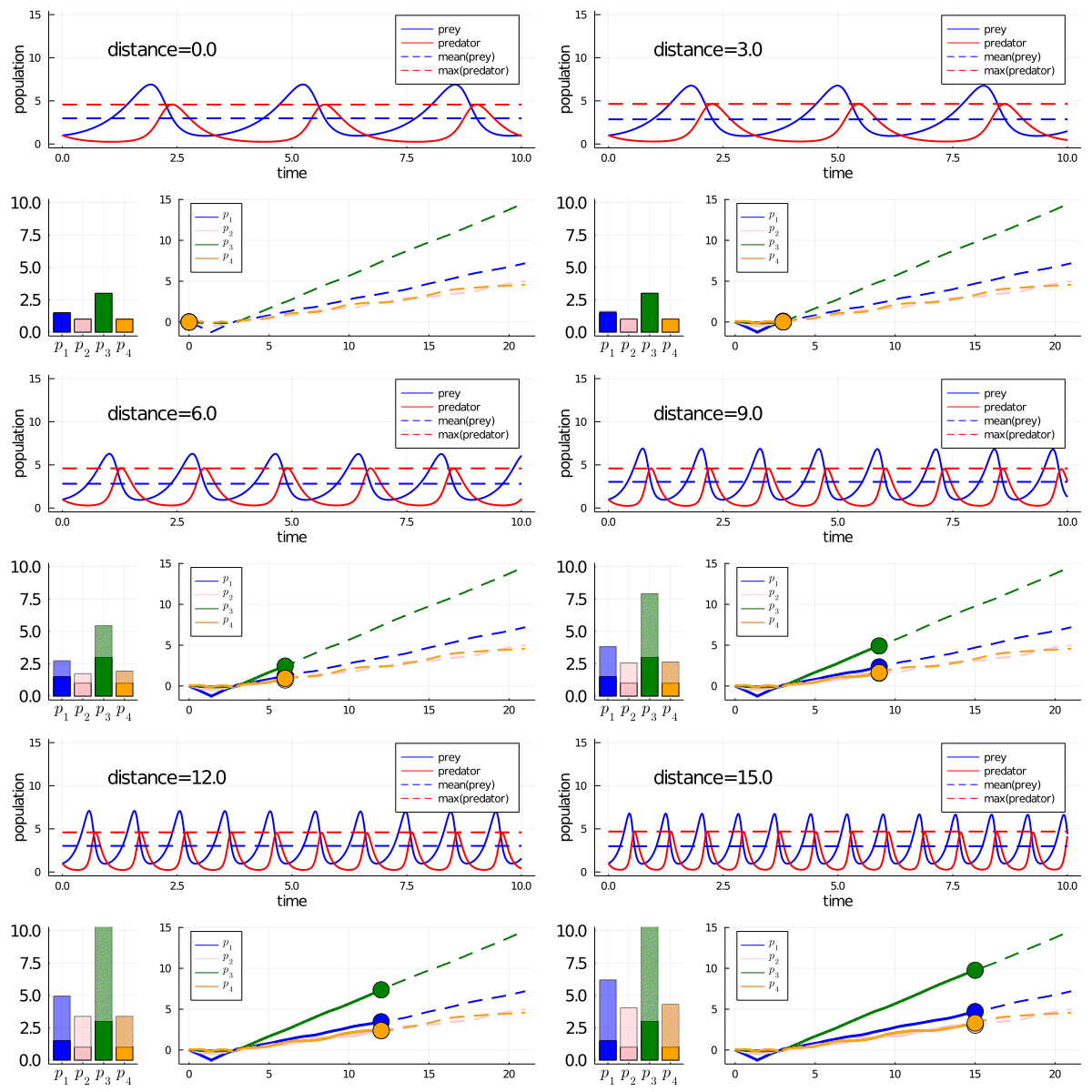
- This curve instead finds a way to modulate the frequency of predator‑predator‑prey interactions while preserving model features.
- Note how it abruptly changes direction when slowing frequency prevents model features from being maintained (as the period approaches the length of the simulation). It goes from decreasing the frequency to increasing it.
The code#
This snippet runs and plots the MDCs
using LinearAlgebra, OrdinaryDiffEq, MinimallyDisruptiveCurves, Statistics, Plots, ForwardDiff, LaTeXStrings

# Which eigenvector (direction) to explore along the manifold
# Change this to 1 or 2 to generate the different MDCs discussed above!
which_dir = 1

# ====================================================================
# --- Core Physics Engine (Lotka-Volterra) ---
# ====================================================================

function lotka_volterra_dynamics!(du, u, p, t)
    du[1] = p[1] * u[1] - p[2] * u[1] * u[2]
    du[2] = -p[3] * u[2] + p[4] * u[1] * u[2]
    return nothing
end

u0 = [1.0, 1.0]
tspan = (0.0, 10.0)
p_nominal = [1.5, 1.0, 3.0, 1.0]

nom_prob = ODEProblem(lotka_volterra_dynamics!, u0, tspan, p_nominal)

# Helper for evaluations
solve_at_p(p) = solve(remake(nom_prob; p = p), Tsit5())

# ====================================================================
# --- Objective Features & Cost Framework ---
# ====================================================================

function extract_features(p)
    sol = solve_at_p(p)
    grid = range(0.0, 10.0, length = 200)

    # Efficient lazy evaluations utilizing solution interpolation
    mean_prey = mean(sol(t)[1] for t in grid)
    max_predator = maximum(sol(t)[2] for t in grid)

    return [mean_prey, max_predator]
end

nom_features = extract_features(p_nominal)

function loss(p)
    p_features = extract_features(p)
    return sum(abs2, p_features .- nom_features)
end

function loss_grad!(g, p)
    ForwardDiff.gradient!(g, loss, p)
    return g
end

core_cost = CostFunction(loss, loss_grad!)

# ====================================================================
# --- Execution Pipeline ---
# ====================================================================

println("--- Setting up Lotka-Volterra MDC System ---")

# Compute the local Hessian at nominal parameters to discover insensitive directions
hess0 = ForwardDiff.hessian(loss, p_nominal)
eigen_decomposition = eigen(hess0)
init_dir = eigen_decomposition.vectors[:, which_dir]

# Leverage our automated IdentityTransform fallbacks to keep the top layer clean
sys = MDCProblem(
    core_cost,
    p_nominal,
    init_dir,
    1.0;                  # Energy Headroom (H)
    names = [:p₁, :p₂, :p₃, :p₄]
)

println("Launching parallel manifold integration...")
mdc_curves = MDCSolve(sys, span = MDCSpan(-1.0, 5.0))

plot(mdc_curves)
The next snippet uses our animation methodology to get a nice animation. All you need to provide is a function (lotka_volterra_sandbox_painter in this case) that goes from parameters to a drawing of your simulation.
# ====================================================================
# --- Animation Pipeline Integration ---
# ====================================================================

println("\nPreparing continuous manifold animation...")

# Define the live sandbox rendering function
function lotka_volterra_sandbox_painter(θ_physical)
    plot_t_grid = range(tspan[1], tspan[2], length = 200)

    sol_nominal = solve_at_p(p_nominal)
    sol_perturbed = solve_at_p(θ_physical)

    states_nom = [sol_nominal(t_val) for t_val in plot_t_grid]
    states_pert = [sol_perturbed(t_val) for t_val in plot_t_grid]

    prey_nominal = [u[1] for u in states_nom]
    pred_nominal = [u[2] for u in states_nom]

    prey_perturbed = [u[1] for u in states_pert]
    pred_perturbed = [u[2] for u in states_pert]

    mean_prey_nom = mean(prey_nominal)
    mean_prey_pert = mean(prey_perturbed)
    max_pred_nom = maximum(pred_nominal)
    max_pred_pert = maximum(pred_perturbed)

    Plots.plot!(
        plot_t_grid, [prey_nominal pred_nominal],
        subplot = 1,
        linealpha = 0.2, linestyle = :dash,
        color = [:blue :red], label = false
    )

    Plots.plot!(
        plot_t_grid, [prey_perturbed pred_perturbed],
        subplot = 1,
        linewidth = 2,
        color = [:blue :red], label = ["Prey (x)" "Predator (y)"],
        legend = :topright
    )

    Plots.hline!([mean_prey_nom], subplot = 1, linestyle = :dot, linealpha = 0.4, color = :blue, label = false)
    Plots.hline!([max_pred_nom], subplot = 1, linestyle = :dot, linealpha = 0.4, color = :red, label = false)

    Plots.hline!([mean_prey_pert], subplot = 1, linestyle = :dashdot, linewidth = 1.2, color = :darkblue, label = "Mean Prey")
    Plots.hline!([max_pred_pert], subplot = 1, linestyle = :dashdot, linewidth = 1.2, color = :darkred, label = "Max Predator")

    return Plots.plot!(
        subplot = 1,
        xlabel = "Time", ylabel = "Population",
        xlims = tspan,
        ylims = (0.0, 6.0)
    )
end

# Invoke the updated linear animation tracking utility function
lv_animation = animate_mdc(
    mdc_curves,
    lotka_volterra_sandbox_painter;
    fps = 20,
    density = 150,
    raw = true
)

output_path = joinpath(pwd(), "lotka_volterra_mdc.gif")
println("Rendering frames and saving video to: $output_path")
Plots.gif(lv_animation, output_path)Lessons#
MinimallyDisruptiveCurves.jl showed how we could continuously vary the parameters of the Lotka‑Volterra model while preserving
- mean prey population over time, and
- max predator population over time.
One strategy (MDC 1) was to alter the parameters to increase (decrease) birth and death rates of the predators while decreasing (increasing) of the prey. Along the \(r\)‑to‑\(K\) axis this corresponds to one species moving in one direction while the other moves in reverse.
Another strategy (MDC 2) was to modulate the frequency of the oscillations. MDC 2 showed us exactly how to change the parameters to continuously modulate this frequency.
By the way
The maximum predator population over time is a non‑differentiable function of the solution. How come this worked?
- ReLU units in neural networks are also technically nondifferentiable a single point, yet they are used successfully in differentiable machine‑machine‑learning models. Same reason!
- The maximum of a collection of values is differentiable except at points where two values tie for the maximum. Numerical error and the dynamics of the ODE ensure that exact ties never occur, so the gradient well‑defined in practice.
Scripts#
If you clone the package itself, it contains some didactic example scripts that show how to build differentiable cost functions out of differential equation models (including those built with ModelingToolkit.jl v11), and extract insight from the underlying models. Specifically, in the terminal:
- Clone the package (
git clone https://github.com/SciML/MinimallyDisruptiveCurves.jl.git)
git clone https://github.com/SciML/MinimallyDisruptiveCurves.jl.git- Move to root directory:
cd MinimallyDisruptiveCurves.jl- Run Julia from the terminal in the package directory as:
julia --project=scriptsThen in the julia REPL that opens, you can run the scripts as follows:
include("scripts/basic_mass_spring.jl") # most basic example on a damped mass spring model
include("scripts/basic_lotka_volterra.jl") # adds one level of complexity: finding good initial curve directions.
include("scripts/frozen_mtk_loss_test.jl") # simple example of how to make a differentiable cost function on an ODE built with ModelingToolkit.jl. No MDC involved!
include("scripts/lotka_volterra_optim.jl") # same lotka volterra model, this time built with ModelingToolkit.jl
include("scripts/build_NFKB.jl") # more complicated model built with ModelingToolkit.jl. more advanced initial curve direction generation. shows how to get real mechanistic insight with the package.
include("scripts/mass_spring_transforms.jl") # how to use the `TransformChain` functionality to manipulate your parameter space for more insightful MDCs
include("scripts/basic_mass_spring.jl")
include("scripts/basic_mass_spring.jl")
Pluto Notebooks#
These use the deprecated version of the package for now. So old syntax. But the didactic flow could be useful, and is similar. Has
- Basic tutorial with mass spring oscillator
- Extracting mechanistic insight from an NFKB model
- Extracting mechanistic insight from a Circadian Oscillator model
Another notebook using the deprecated package version but that’s interesting is https://github.com/Dhruva2/MDCExamples/blob/master/calcium_homeo.jl
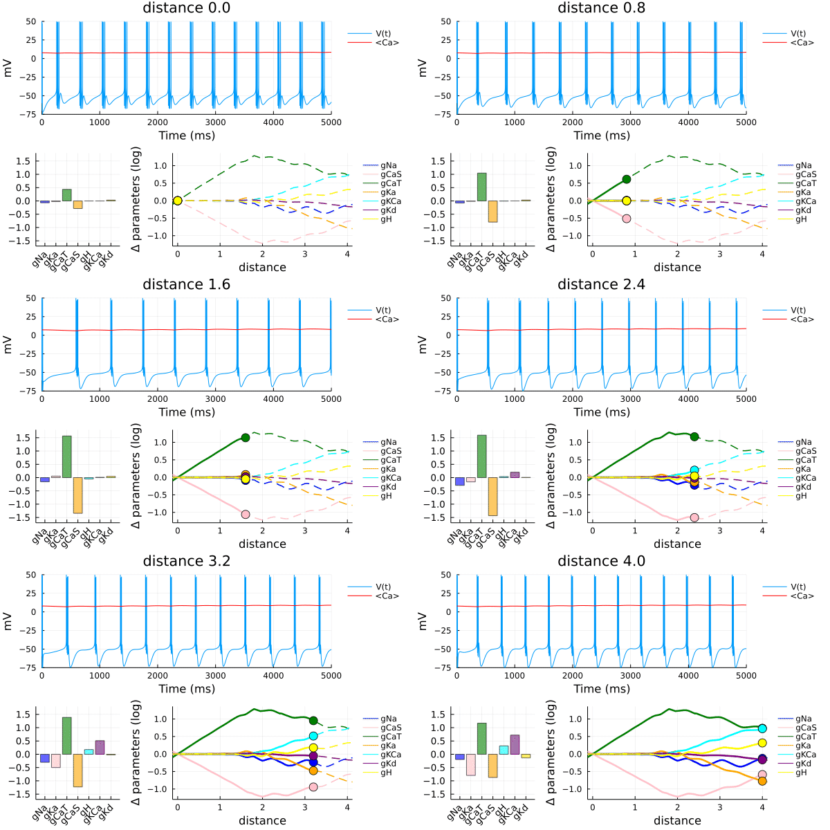
(Built by Andrea Ramirez Hincapie). I’m a calcium-sensitive bursting neuron model. I have to modulate my electrical activity (e.g. from spiking to bursting). I also have to maintain calcium homeostasis: internal calcium concentration needs to be in a tight range for me to be happy. But changing baseline electrical activity changes baseline calcium! How can I safely neuromodulate, while preserving calcium concentration? MDCs tell me how…
It leads up to generating: