How it works#
Notation#
- Let’s say our model has \(N \) parameters.
- The set of allowable parameter values is denoted \(\Theta \subseteq \mathbb{R}^N \). For instance, maybe parameter values must be positive, in which case \(\Theta \) is the positive orthant.
- Any particular model configuration can be defined by a vector of \(N \) parameters: \(\theta \in \Theta \).
- We denote the cost (loss) function as
$$ C: \Theta \to \mathbb{R}. $$
\(C(\theta)\ \) tells us “how badly’’ the model behaves when using the parameter vector \(\theta \). The smaller \(C(\theta) \) is, the better the model behaves.
Background: model‑fitting#
Let’s quickly recap the problem of model‑fitting (optimising the model), and define some notation for subsequent use.
Graphically#
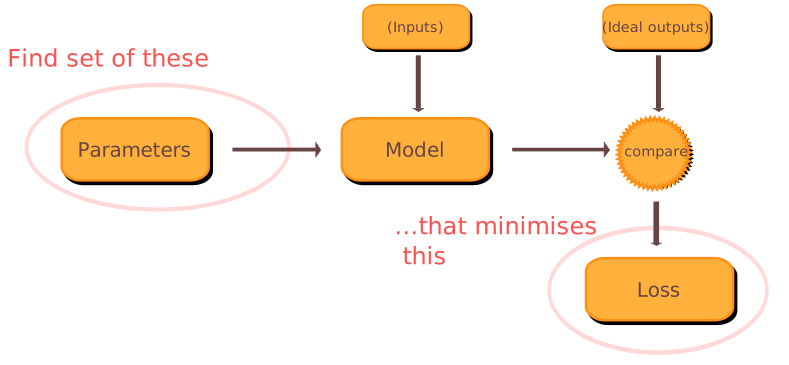
(bracketed blocks are optional. Ideal outputs could be experimental data)
But we can abstract away fixed blocks to get our cost function:

Verbally#
- When we make a model of a system, we want it to recreate some desired behaviour(s).
- To do so, we make a cost (also called loss) function, that takes in model behaviour, and spits out how bad it is. Larger loss ⇒ less model behaviour.
- Of course, the modeller has to define the measure of bad behaviour. For instance, squared deviation from data the model is supposed to fit (is used too much).
By the way
- Most systems one would model in Biology and Engineering (my interests) are input‑output systems. You turn the steering wheel, the car veers. You inject current, the neuron fires. You add a cytokine, the cell’s system responds.
- Therefore reasonable cost functions should penalise bad model behaviour for multiple inputs. I want my car to turn left when I steer left. I also want my car to turn right when I steer right.
- Don’t conveniently forget this to make the modelling/analysis easier. Too many biological models do. I’m also guilty.
MinimallyDisruptiveCurves.jlallows you easily sum multiple cost functions (one for each input). It evaluates them in a multithreaded way, so that performance doesn’t take such a hit.
Mathematically#
Model fitting (also known as training, optimisation, calibration, …) is running
$$ \theta^{*} = \arg\min_{\theta} C(\theta) $$
subject to \(\theta \in \Theta \).
- Since \(C(\theta) \) is a scalar function (returns a scalar), we can think of it as a landscape, where height is analogous to \(C(\theta) \), and lateral co‑ordinates are the parameters \(\theta \) of the problem. Then model fitting is just finding a path to the deepest point of the landscape! (see below)
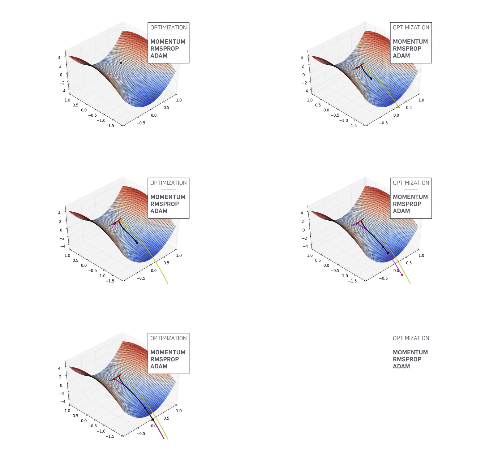
*This gif was taken from an Intro to Optimization blog post, [website herehere](https://blog.paperspace.com/intro-to-optimization-momentum-rmsproph
What are we trying to do#
Recall the goal. Given a fitted model, we want to:
Find functional relationships between model parameters that best preserve model behaviour.
To do this, our curve generator wants to
get as far away as possible from the initial parameters, while keeping the cost function as low as possible.
By the way
- Optimisation consists of descending to the lowest point of the cost landscape (without worrying about your particular trajectory).
- We, on the other hand, are trying to flow along the valleys of the landscape. Like a river. But one that has enough energy to go uphill to a specified elevation (the momentum parameter) if it can’t find a flat/flat/downhill direction.
Let’s express this mathematically. We can define a curve on parameter space as a function
$$ \gamma : [0,F] \to \Theta . $$
The input \(s\in[0,F] \) to the curve is a scalar number that specifies ““how far along’’ the curve we are. So \(\gamma(0) \) is the initial point, and \(\gamma(F) \) is the final point.
Any point \( \gamma(s) \) on the curve has a derivative, \(\gamma’(s) \). This is the direction in which it is pointing (i.e. the direction of the tangent). Let’s fix
- \(\gamma(0)=\theta^{*} \), the locally optimal parameter vector gained from model fitting.
- \(\gamma’(0) \), the initial starting direction of the curve, as a user‑user‑defined parameter.
We will denote the set of allowable curves \(\gamma \) (i.e. those satisfying the above constraints) as \(\Gamma \).
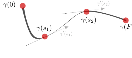
By the way
We are going to iteratively add constraints to the set of allowable curvescurves, and thus shrink \(\Gamma \).
Now we want all points on our curve to define low‑cost parameter configurations. In other words, we want \(C(\gamma(s)) \) to be small for any \(s\in[0,F] \). How can we distinguish between “good’’ and “bad’’ curves? How about this:
$$ J[\gamma] = \int_{\gamma} C[\gamma(s)] , ds $$
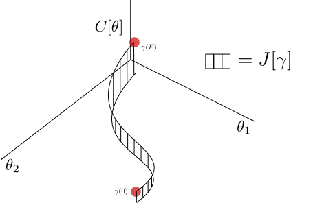
\(J \) is the line integral of the cost \(C \) along the curve \(\gamma(\gamma \). If \(J[\gamma] \) is small, then \(C \) is necessarily small along the entire curve.
By the way
Vector calculus 101: we can expand out the line integral as
$$ \int_{\gamma} C[\gamma(s)] , ds = \int_{0}^{F} C[\gamma(s)] , |\gamma(s|\gamma(s)|_{2} , ds . $$
So now the best curve would be the solution of
$$ \min_{\gamma\in\Gamma} J[\gamma] . $$
But wait!
What’s preventing the curve from just buzzing around \(\gamma(0)=\theta(\gamma(0)=\theta^{*} \). Since we know that \(C(\theta^{*}) \) is as low as can be?
Absolutely nothing!
So let’s add a constraint that the direction of the curve must always be pointing away from \(\theta^{*} \). Mathematically:
$$ \frac{d}{ds},|\gamma(s)-\theta^{*}|_{2} > 0,\qquad \forall s\in[0,F]. $$
But wait again!
What if the curve “doesn’t want to evolve’’ because every direction increases the cost. So it just…stays short.
Absolutely nothing again!
We want a curve that actually changes the parameters appreciably. So let’constrain the length of the curve, by setting how fast it moves as a function of \(s \):
$$ |\gamma’(s)|_{2}=1\qquad \forall s\in[0,F]. $$
Now the curve has to have length \(F \).
So to wrap up, our allowable set of curves $$\Gamma = \gamma:[0,F]\to\Theta $$ satisfies
$$ \begin{aligned} & \frac{d}{ds}|\gamma(s)-\theta^{*}|_{2}>0; \\ & \gamma(0)=\theta^{*}; \\ & | \gamma’(s) |_2 = 1 \\ & \gamma’(0)=\delta\theta^{*} \end{aligned} $$
for some fixed initial direction \(\delta\theta^{*}\in\mathbb{R}^{N} \). Our mathematical problem is
$$ \min_{\gamma\in\Gamma} J[\gamma],\qquad J[\gamma]=\int_{\gamma} C[\gamma(s)],ds . \tag{1} $$
How we do it#
If equation \((1) \) reminds you of a variational‑calculus problem, you would be right! Now we just have to solve the Euler‑Lagrange equations, right?
Wrong. It’s too hard! Try it yourself if you want. I’m not going to explain why … lots of potential curves, not so many constraints.
So instead of searching directly over curves, we are going to turn this into a dynamic problem. Stop thinking about curves as static shapes. thinking about curves as things that are drawn over time.
This turns it into an optimal‑control problem:
- Imagine a rocket sitting at \(\theta^{*} \).
- It needs to traverse a trajectory in parameter space.
- At each point in time, we send it a control input, that determines its current direction (i.e. we steer the rocket).
- Problem: Design a steering law so that the trajectory traced by rocket is a (locally) optimal solution of equation \((1) \).
By the way
- The rocket analogy is there for a reason. Optimal‑control theory got going in the 1950s, when the USSR and the USA suddenly got interested in designing aircraft/rocket trajectories that were optimal for doing military things. No prizes for guessing why.
- Here’s a history
- Two solutions emerged, separated by the Iron Curtain: Pontryagin’s maximum principle, and Bellman’s principle of optimality.
- Using one of these methods, we shall seize the means of curve generationgeneration, Comrade!
Let us mathematically express equation \((1) \) as an optimal‑control problem:
- At each time \(t \) we choose an input \(u(t) \). The whole trajectory, from \(t=0 \) to \(t=F \), we denote \(u \). The space of possible trajectories is \(\mathcal{U} \). So \(u\in\mathcal{U} \).
- The dynamics of the “rocket’’ are \(\theta’(t)=u(t) \) (i.e. we directly control rocket velocity).
- By transcribing the constraints on \(\gamma’(s) \) in the previous section to constraints on \(u(s) \), we define the space of possible input trajectories as
$$ \mathcal{U}= \Big\{u:|u(t)|_{2}=1; \langle u(t),\gamma(t)-\theta^{*} \ u(t),\gamma(t)-\theta^{*}\rangle\ge 0; u(0)=\delta\theta^{*};\forall t\in[0,F]\Big\}. $$
- Our minimisation problem \((1) \) is now
$$ \min_{u\in\mathcal{U}} J(u),\qquad J(u)=\int_{\gamma} C,d\gamma,;; \gamma’(t)=u(t),;\forall s\in[0,F]. $$
You can then apply Pontryagin’s maximum principle to get some complicated constraints on \(u(s) \).
By the way
- Usually, solving the optimal‑control problem using Pontryagin’s maximum principle requires solving a boundary‑value problem. These are annoying solve.
- Luckily, by tinkering with constraints (see PhD‑thesis reference), we factor out the boundary constraints, and end up with an explicit ordinary differential equation that defines optimal curve evolution.
Now, we are going to write down the differential equations for curve evolution
- They are complicated and you should feel free to skip them. Intuition will be provided subsequently.
Pontryagin’s maximum principle requires dynamics for not only the state of the system (i.e. the position \(\gamma(s) \) of the rocket) but also the costate of the system. What is this? Something roughly analogous to the momentum of the rocket, but also affected by all the input constraints we have set.
So we get two curves. One for the state \(\gamma(s) \), and the other for the costate, which we shall denote \(\lambda(s) \).
- Let \(H:=C[\gamma(F)] \) be the final cost. We set this a priori as a hyper‑parameter. Curve evolution stops prematurely if \(C[\gamma(s)]\ge HH \).
By the way
- Pre‑setting \(H \) is the trick that turns this from a boundary‑value problem into a (much easier) ODE problem.
- Let \(\mu_{2}(s)=\dfrac{C[\gamma(s)]-H}{2} \).
- Define \(\mu_{1}(s)\ge0 \) and impose the constraint \(\mu_{1}(s)\u(s),\gamma(s)-\theta^{*}\rangle =0 \).
- Let \(\lambda(0)=\big(H-C[\gamma(0)]\big)u(0) \).
Then
$$ \lambda’(s)=\mu_{1}(s)u(s)-\nabla_{\theta}C[\gamma(s)], \qquad \gamma’(s)=u(s), \qquad u(s)=\frac{\lambda(s)-\mu_{1}(s)[\gamma(s)-\theta^{*}]}{2\mu_{2}(s)} . $$
Given \(C[\gamma(s)] \) (the current cost) and \(\nabla_{\theta}C[\gamma(s(\nabla_{\theta}C[\gamma(s)] \) (its gradient), we can solve these as a coupled ODE system for \(\gamma(s) \) and \(\lambda(s) \).
By the way
- Get some intuition by setting \(\mu_{1}(s)=0 \) in your head, then reviewing the equations. This occurs when the curve is currently pointing away from \(\theta^{*} \).
- Then you see that \(u(s) \), the curve direction, is proportional to \(\(\lambda(s) \), the costate (≈ momentum).
- Meanwhile, the costate is integrating the negative cost gradient, \(-\nabla_{\theta}C[\gamma(s)] \).
- Notice the analogy with optimisation algorithms based on gradient descent with momentum, if you’re into that kind of thing.
TL;DR#
What we are trying to do
We wanted a method to construct curves in parameter space, where
- Every point on the curve represents a set of model parameters that is low‑cost as possible.
- The curves don’t “double back’’ on themselves (monotonically increasing distance from the origin).
- The curves have a fixed length \(F \).
- The user sets the initial direction of the curve.
This resulted in the optimisation problem of equation \((1) \).
How we do it
To make solution of this variational problem tractable, we turned it into an optimal‑control problem.
- We made the analogy of a rocket, with an automatic steering law, traversing parameter space.
- We asked what steering law would result in a rocket trajectory corresponding to a curve satisfying the above requirements.
This resulted in a set of differential equations that evolve paired ““position’’ and “momentum’’ variables for the rocket. Position represents the point on parameter space (i.e. the curve).
- Solving this differential equation requires evaluation of the cost function and its gradient at every step.