MinimallyDisruptiveCurves.jl#
Because building a good model is hard#

But extracting useful insight from it is harder#
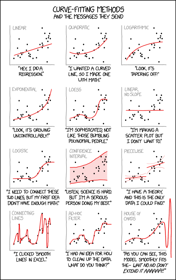
(Credit: https://xkcd.com/793/ and https://xkcd.com/2048/)
What it does (short form)#
At its core, only one thing:
Finds the hidden, potentially nonlinear relationships between model parameters that best preserve user‑defined features of model behaviour.
(…by solving a differential equation on the parameters)
Explanation by example#
- This is the four‑parameter Lotka‑Volterra differential‑equation model predator‑prey dynamics. Covered in more detail in Examples
$$ \begin{aligned} \frac{d\text{🐁}}{dt} &= p_1\text{🐁} - p_2 \text{🦉} \text{🐁} \\ \frac{d\text{🦉}}{dt} &= -p_3\text{🦉} + p_4 \text{🐁} \text{🦉} \end{aligned} $$
(🐁 are born at rate \(p_1\), die/are eaten at rate \(p_2\). 🦉 die at rate \(p_3\), are born at rate \(p_4\).)
- Model dynamics at
p = [1.5,1.0,3.0,1.0]):
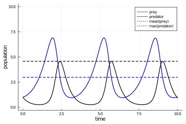
We quantify good model behaviour as having a particular, fixed value for
- mean prey population over time
- max predator population over time
Each minimally disruptive curve finds a different way to change parameters while “minimally disrupting’’ these model features:
MDC 1
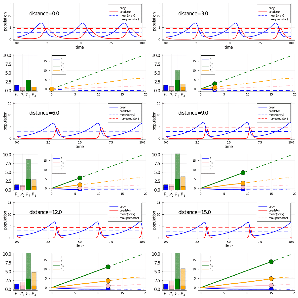
MDC 2
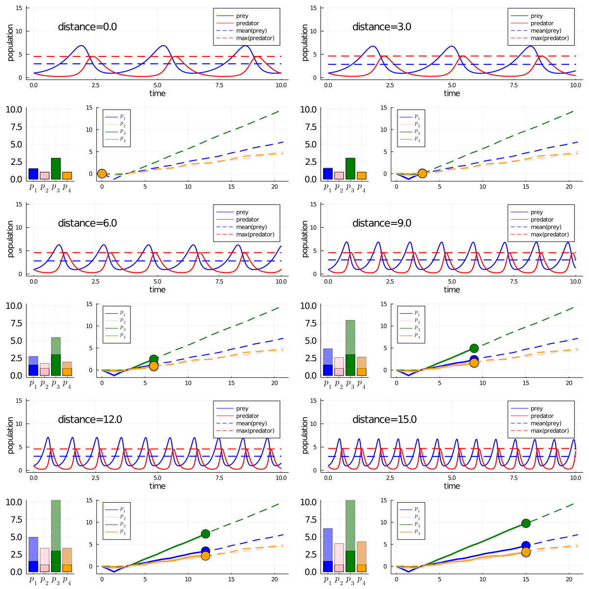
Both curves evolved in seconds on a laptop.
MDC generation was automatic – no human insight required!
Want more involved examples?
Check out the examples in the docs.
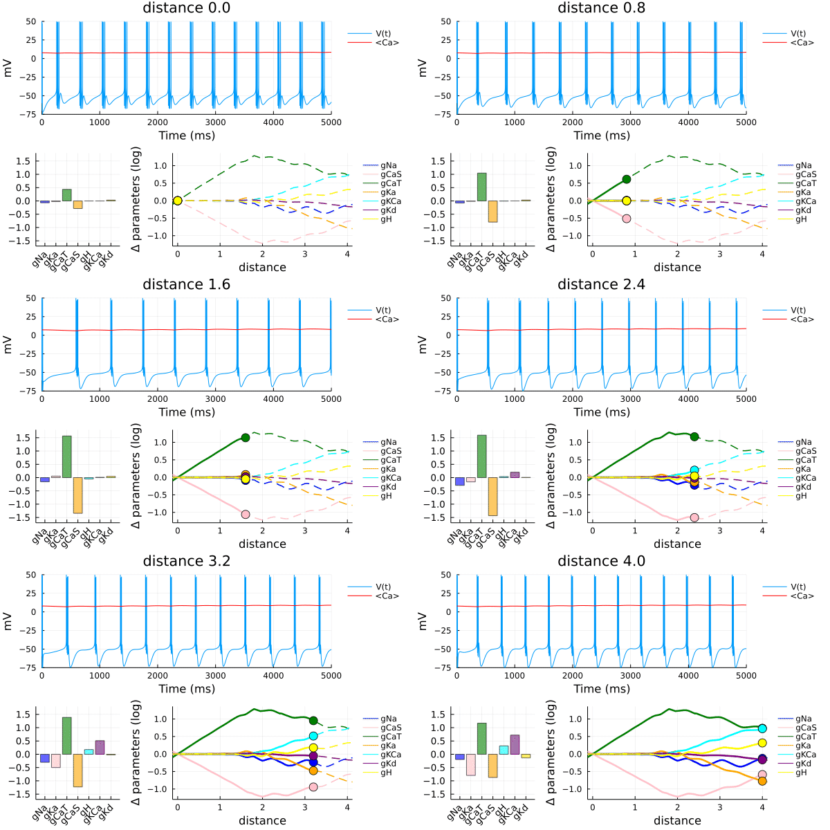
Here is a teaser: parameter relationships on a model of a bursting neuron that preserve its physiological, time‑averaged calcium concentration, and the “bursting’’ phenotype of its voltage trace. Parameters are the ion‑channel densities, which are physiologically variable.
Schematic#
Minimally disruptive curve
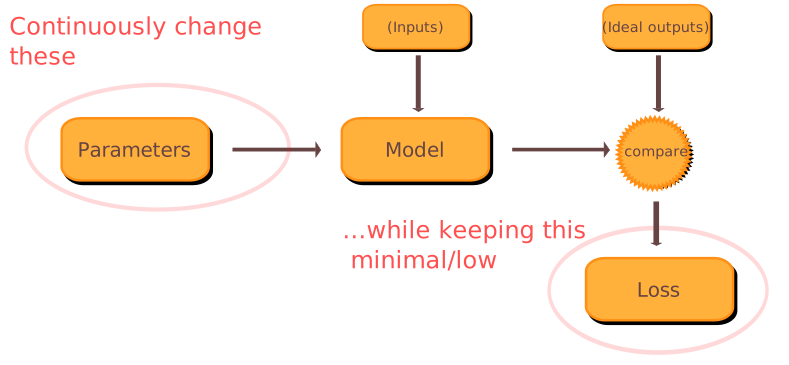
(bracketed blocks are optional. Ideal outputs could be experimental datadata.)
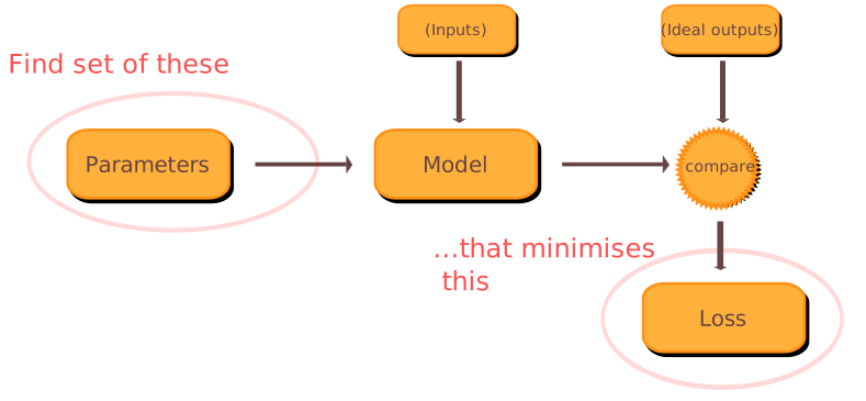
Compared to model fitting/optimisation (which this is not)
You start with an initial set of parameters for which the model “works’’ as you want (as quantified by a cost/loss function). You can get this from model fitting/optimisation.
Each minimally disruptive curve is a continuous path in parameter space; any point on path yields parameters that still (nearly) work.
The job of the MD‑curve generator is to
get as far away as possible from the initial parameters, while keeping the cost function as low as possible.
By the way
- As far away as possible implies some notion of distance (metric) on parameter space. Maybe you’re interested in relative, rather than absolute changes. Or you’re particularly interested in changes to a few particular parameters. MinimallyDisruptiveCurves.jl makes it easy to make your own custom metric (see Features section).
By the way
Play around with curve specifications such as :
- the initial curve direction
- which parameters the curve can(not) change
- which parameters the curve is biased towards changing
- reparameterising the cost function
… to get different minimally disruptive curves yielding different model insights.
Not happy with the explanation? See the following sources for more information:
| Source | Rigorous enough | Excessively rigorous | Excessively verbose | Unreliable |
|---|---|---|---|---|
| My thesis, ch. 5 (ch. 4 is relevant too) | x | x | ||
| Raman et al. 2017 | x | x | ||
| How it works | x | |||
| dvr23@cam.ac.uk | x |
Use Cases#
You have a differentiable mathematical model, and want to answer questions like:
- Which model interactions could I kill without greatly affecting model behaviour?
- Is there a hidden approximation I could make in the model that wouldn’t greatly change behaviour?
- Are model parameters structurally / practically identifiable from data? If not, which (functions of the) parameters are unidentifiable?
- (Dually) What spaces of parameters are (approximately/exactly) consistent with the data / desired behaviour?
- Could changes in parameter \( x \) be continuously compensated for by changes in parameters \( y \) and \( z \)? Or by \( u \), \( v \), and \( w \)? Or by any parameters at all? If so, what kind of compensatory changes?
By the way
- We provide Examples in which MD curves answer all of the above questions
(on differential equation models from systems biology/neuroscience due to author prejudice. The package is model‑agnostic.) - If you find any other use case, let me know!
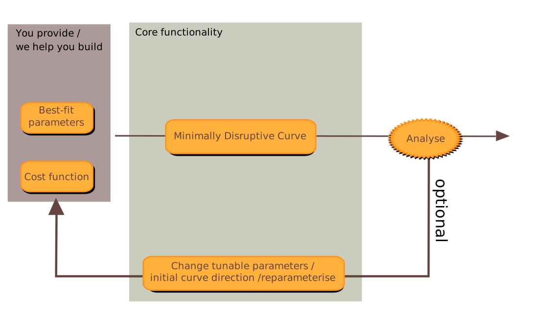
Basic workflow#
By the way
- MinimallyDisruptiveCurves never interacts directly with your model. Only the cost function. So it is agnostic to the model / how you coded the model.
- Your cost function can be anything, as long as it’s differentiable. Quantify how well the model matches data, oscillates at 4 Hz or does backflips. Your choice.
What you need
- A Julia function (the cost function) with two methods as shown:
# 1. The cost function (returns a scalar)
function cost(params)
  …
  return cost_value
end

# 2. The in-place gradient function (mutates g)
function grad!(g, params)
  …
  g .= ∇C(params)  # MUTATE the gradient holder.
  return g          # The package ignores the return value, but returning `g` is good Julia convention.
end

# 3. Wrap them into a CostFunction
core_cost = CostFunction(cost, grad!)

# 4. OPTIONAL: Wrap in a TransformedCost to explore relative/log space,
# bias parameters, or fix certain parameters.
# If omitted, MDCProblem will automatically use an empty TransformChain.
chain = TransformChain(LogAbsTransform())
transformed_cost = TransformedCost(core_cost, chain)

# 5. Pass to the MDCProblem
sys = MDCProblem(transformed_cost, p0, dp0, mom)- An initial set of parameters,
p0, that are locally minimal (or close enough) with respect to the cost function. So
grad_holder = rand(size(p0))
c0 = cost(p0, grad_holder)
# now grad_holder ≈ zeros(size(grad_holder))- How do you get such a
p0? By fitting the model to the cost function. In Julia, you can choose from a variety of optimisation packages. I use Optim.jl in the examples.
By the way
Calculating the gradients of cost functions of complicated models is hard right?
Not these days! Automatic differentiation of near‑arbitrary code is one of the big advantages of Julia. See the Examples. Also note
- The two‑method specification of the cost function above is shared with most Julia optimisation packages (e.g. Optim.jl).
- DiffEqParamEstim.jl makes cost functions of the required form for differential‑equation‑based models.
- Otherwise, Zygote.jl and ForwardDiff.jl can collectively take the gradient of pretty much any differentiable Julia code.
- If all else fails, MinimallyDisruptiveCurves.jl provides a helper:
make_fd_differentiable(cost), which spits out a finite‑difference gradient version. But using finite‑difference differentiation with Julia is like using a Ferrari to do the school run.
An initial curve direction
dp0.- You can find the minimally disruptive initial direction using local sensitivity analysis. MinimallyDisruptiveCurves.jl has tools to help you with that. Or you can find a custom direction involving a few parameters you are interested in.
A momentum hyper‑parameter:
mom, with a default value. The curve stops evolving once \( C(p) \geq mom \).
Then you can run the following code:
# span defines the length of the curve in the negative and positive directions.
# Negative values ⇒ two curves are evolved in parallel, in the directions ±dp0,
# with lengths span[1] and span[2].

sys = MDCProblem(cost, p0, dp0, mom)
# create an object that stores all the curve information

mdc_curves = MDCSolve(sys; span=MDCSpan(-50.0, 100.0))   # solve the ODE that evolves the MD curve
using Plots
plot(mdc_curves)   # custom plotting of the important features of the MD curve.```


`mdc` is a `MDCSolution`. This type comes with functionality for inspecting / interpolating the curve at different points – all hijacked from DifferentialEquations.jl, of course.


## Features

**Code whatever model you like, however you like**
- MinimallyDisruptiveCurves.jl does not directly interact with your model. You only need to provide a cost function as described above. Hence there is no constraint on the model simulation step inside the cost function. You could even have your model simulation in another language and call it via `pycall.jl` or `ccall.jl`.

**Avoids the curse of dimensionality**
- Because the package is not based on sampling parameter space, it does not suffer from the curse of dimensionality in models with many parameters.
- Generating a minimally disruptive curve usually requires somewhere between a few hundred and a few thousand evaluations of your cost function (and its gradient). That is the major computational cost.
- If you use reverse‑mode automatic differentiation to compute your cost gradient, the computational complexity of gradient evaluation grows favourably with the number of parameters. That is why machine‑learning models with millions of parameters optimise so fast.

**Multithreaded cost‑function summation**
- Often you want a model to behave one way for one input, and another way for another input. Each case induces a separate cost function. You can sum cost functions with `sum_losses(arr)`, where `arr` is an array of cost functions. The resulting summed cost function runs each component cost on a separate thread, giving an efficient overall cost evaluation.

**Easily manipulate cost functions**
- Many MinimallyDisruptiveCurves.jl workflows require regularly fixing / freeing cost‑function parameters, or completely reparameterising cost functions.
- For example, you might be interested in only allowing a few parameters to change, or you might want to bias the curve to align with a particular parameter.
- The package provides composable `AbstractTransform` objects that you chain together into a `TransformChain` to define a transformation

  $$ T : \mathbb{R}^N \to \mathbb{R}^M $$

  from the optimizer space to the physical space. You just wrap your `CostFunction` in a `TransformedCost` along with your chain:

  ```julia
  chain = TransformChain(LogAbsTransform(), ScaleTransform([1.0, 10.0]))
  C_new = TransformedCost(core_cost, chain)

  to obtain a new differentiable cost function \\( \tilde{C} \\) satisfying

  $$ \tilde{C}(T(p)) = C(p). $$

- Pre‑loaded transforms include

  - `LogAbsTransform()`: \\( T = \log \circ |\cdot| \\) for relative‑change‑sensitive parameters.
  - `ScaleTransform(w)`: \\( T : p_i \mapsto w_i\,p_i \\) for biasing towards or away from particular parameters.
  - `FixedParamsTransform()`: Fixing / freeing (all except / only) named parameters.

- The source code for each of these is ≤ 10 lines, so you can easily write your own.


## Caveats

**Your cost function needs to be differentiable.**
- Your cost function is a mathematical expression of what you want your model to do. A little bit of ingenuity can usually find differentiable cost functions that successfully express this
- Otherwise, switch your brain off and take your cost as the L2 deviation from some ideal model output.
- Or finite difference the gradient with `make_fd_differentiable(cost)`, close your eyes, and hope for the best.


**MinimallyDisruptiveCurves.jl generates 1‑D functional relationships (i.e. *curves*).**
- There may be higher-dimensional functional relationships (i.e. surfaces or hyper-surfaces) in parameter space, over which model behaviour is approximately preserved. You won't automatically find these using MinimallyDisruptiveCurves.jl. But by evolving multiple curves with different initial conditions / at different points in parameter space, you could get somewhere.

## Related literature

Not convinced this is the right way to do things? [Raman et al. 2017](https://journals.aps.org/pre/abstract/10.1103/PhysRevE.95.032314) provides a literature review of alternative methods and their relative pros/cons.

## Citing, Acknowledgements

**The algorithm**  (minus a few tweaks)

```bibtex
@article{raman2017delineating,
  title   = {Delineating parameter unidentifiabilities in complex models},
  author  = {Raman, Dhruva V and Anderson, James and Papachristodoulou, Antonis},
  journal = {Physical Review E},
  volume  = {95},
  number  = {3},
  pages   = {032314},
  year    = {2017},
  publisher = {APS}
}
The software – as yet unpublished; keep an eye on this!
Funding – This work was supported by European Research Council grant StG 2016 FLEXNEURO (716643). Thanks!
References#
- Raman, Dhruva V., James Anderson, and Antonis Papachristodoulou. “Delineating parameter unidentifiabilities in complex models.” Physical Review E 95, no. 3 (2017): 032314.