Questions from the audience#

Different goals. Bayesian modelling is attempting to extract a posterior distribution. This characterises the quality of every single parameter combination, relative to some user‑defined measure of “goodness‑of‑fit”.

So in Bayesian modelling, regions of high‑posterior (the “interesting” parameter combinations) correspond to clouds in parameter space that are “likely”, given the data/objectives of the model output.

This suffers from the curse of dimensionality if you have lots of parameters.

Conversely, MinimallyDisruptiveCurves.jl extracts structure from this cloud of “likely” parameters, without entirely characterising the cloud.

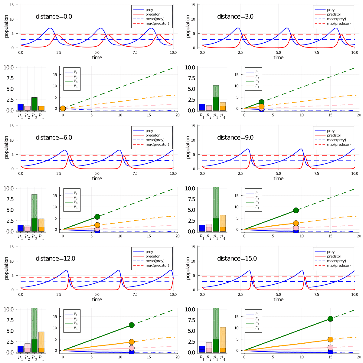
As an example, compare the output of the Bayesian inference on a Lotka‑Volterra example you mentioned (link here) with MinimallyDisruptiveCurves.jl:

• Turing.jl extracts regions of likely parameter values for the model (see the image after plot(chains) in the link).
• MinimallyDisruptiveCurves.jl extracts relationships between parameters over which high likelihood is maintained (see the animation below).

There is a formal correspondence between posterior/likelihood functions and minimally disruptive curves. See Raman et al. (2017) for details.

I certainly think it could be used for social sciences! In particular, the concept of multicollinearity is very important in statistical regression analyses. This is when one regressor variable can be predicted by a linear combination of other regressor variables. It has all sorts of important practical and theoretical consequences on what can (not) be inferred from the model (see the Wikipedia article). Various algorithmic tests exist to detect multicollinearity.

Now, those consequences do not stem from the linearity of the relationship between regressors; they stem from the fact that one can be predicted by the others. Why don’t we test for non‑linear multicollinearity then? Because it’s hard!

…Except this is exactly what MinimallyDisruptiveCurves.jl does!

More generally, conclusions (e.g. health‑risk factors in clinical trials) are often synthesised from the parameter values of models fitted to data. Sensitivity analysis is usually local. A project I want to start is using MDC to find far‑away parameters that still match such data. For instance, if a regression tells me that a dietary feature X increases the risk of cardiac arrest by 10 % over ten years, can I use MDC to find different regression coefficients that change that risk as much as possible while preserving the model fit? If so, the robustness of the conclusion is affected.

Why isn’t MDC.jl used much? I haven’t written a didactic paper explaining the toolbox and its use cases. The paper I did publish was abstract and only presented the algorithm, not an implementation. There may also be methodological flaws I haven’t spotted yet! I’m currently writing a new paper, but MDC is a side‑project for me, so progress is slow.

Any parameter that changes a lot inside a minimally disruptive curve is unidentifiable with respect to the user‑defined cost function. For example, in the Lotka‑Volterra case, all parameters move considerably, so they are effectively unidentifiable with respect to the observed mean prey and maximum predator populations.

The methods of Villaverde et al. look for structurally unidentifiable combinations of parameters. Those correspond to minimally disruptive curves that are “non‑disruptive”, i.e. the cost stays at zero. MDC can also find practically unidentifiable combinations: the cost is not exactly zero but sufficiently small that the practical consequences are the same.

Consider a reaction network with a fast‑timescale reaction parameter that is effectively instantaneous. You can increase this parameter to infinity with almost no effect on the model output—not algebraically zero, but practically negligible. An algebraic tool would not flag this parameter as unidentifiable, whereas MDC.jl would.