Examples

Tutorial notebooks

Tutorial Pluto notebooks are in the MDCExamples repository. Pluto notebooks are like Jupyter notebooks, but (IMO) better for Julia. To install Pluto, open a Julia REPL, and type

]add Pluto
using Pluto
Pluto.run()

Install/open Pluto.jl and copy one of the tutorial URLs into the Pluto search bar. I've put them in a suggested order:

1. https://github.com/Dhruva2/MDCExamples/blob/master/Transformingcostfunctions.jl

• Not about MinimallyDisruptiveCurves specifically, but introduces you to the cost function transformations that are useful when iteratively running MDCs.

2. https://github.com/Dhruva2/MDCExamples/blob/master/massspringintro.jl

• Applying MDCs to the simplest possible differential equation: a damped oscillator. MDC generation happens in the blink of an eye for a model this simple, so it's useful for playing around.

3. https://github.com/Dhruva2/MDCExamples/blob/master/NFKBExample.jl

• Takes a seminal model of the NFkB metabolic pathway. Shows how you can iteratively extract mechanistic insight from the model using MDCs.

4. https://github.com/Dhruva2/MDCExamples/blob/master/CircadianOscillator.jl

• Takes a seminal but rather large model of the intracellular Circadian rhythm. Shows how you can use a 'cheap' loss function (the injection/collocation) loss, to massively speed up MDC generation. The MDCs seem eminently interpretable, but I haven't interpreted them yet. Have a go, if you're a Circadian expert!

5. https://github.com/Dhruva2/MDCExamples/blob/master/calcium_homeo.jl

• (Built by Andrea Ramirez Hincapie). I'm a neuron. I have to modulate my electrical activity (e.g. from spiking to bursting). This is called neuromodulation. I also have to maintain calcium homeostasis: internal calcium concentration needs to be in a tight range for me to be happy. But changing baseline electrical activity changes baseline calcium! How can I safely neuromodulate, while preserving calcium concentration? MDCs tell me how....

A copy-paste, minimal example

• This example is less didactic than the notebooks, but useful for somebody who just wants to get things working quickly.

• We do a cursory analysis of the Lotka-Volterra, predator-prey differential equation model. This is often used as a toy example for global sensitivity analysis tools, see e.g. the following web links: a, b, c. Because it's really simple.

• You can copy and paste the code at the bottom, and run it as a .jl script. It runs in seconds (after package/function pre-compilation). Just make sure you add all the package dependencies first:

] add OrdinaryDiffEq, ForwardDiff, Statistics, Plots, LinearAlgebra, LaTeXStrings
] add https://github.com/Dhruva2/MinimallyDisruptiveCurves.jl.git

• Note that one of the model features we analyse is non-differentiable. Mathematically. Computationally everything works fine, as we'll explain.

Lotka Volterra model of predator-prey interactions

The dynamics for the system are:

$\frac{d 🐁}{dt} = p_1 🐁 - p_2🐁 🦉 \\ \frac{d 🦉}{dt} = -p_3🦉 + p_4 🐁 🦉$

• $p_1$ and $p_2$ are the birth and death rates of 🐁

• $p_3$ and $p_4$ are the birth and death rates of 🦉

... and here is a time-course of their populations when p = [1.5,1.0,3.0,1.0]. We call these values the nominal parameters.

Nominal system (i.e. simulated with nominal parameter values)

• We will follow b in having two features of interest:

  • mean population of 🐁 over time

  • max population of 🦉 over time

• The model features of the nominal system are $[2.98, 4.57]$

• Our cost function on model behaviour is the mean square deviation from these nominal model features.

• By running the code at the bottom of the page twice, setting whichdir = 1 and whichdir=2 respectively, we get two MD curves (see below).

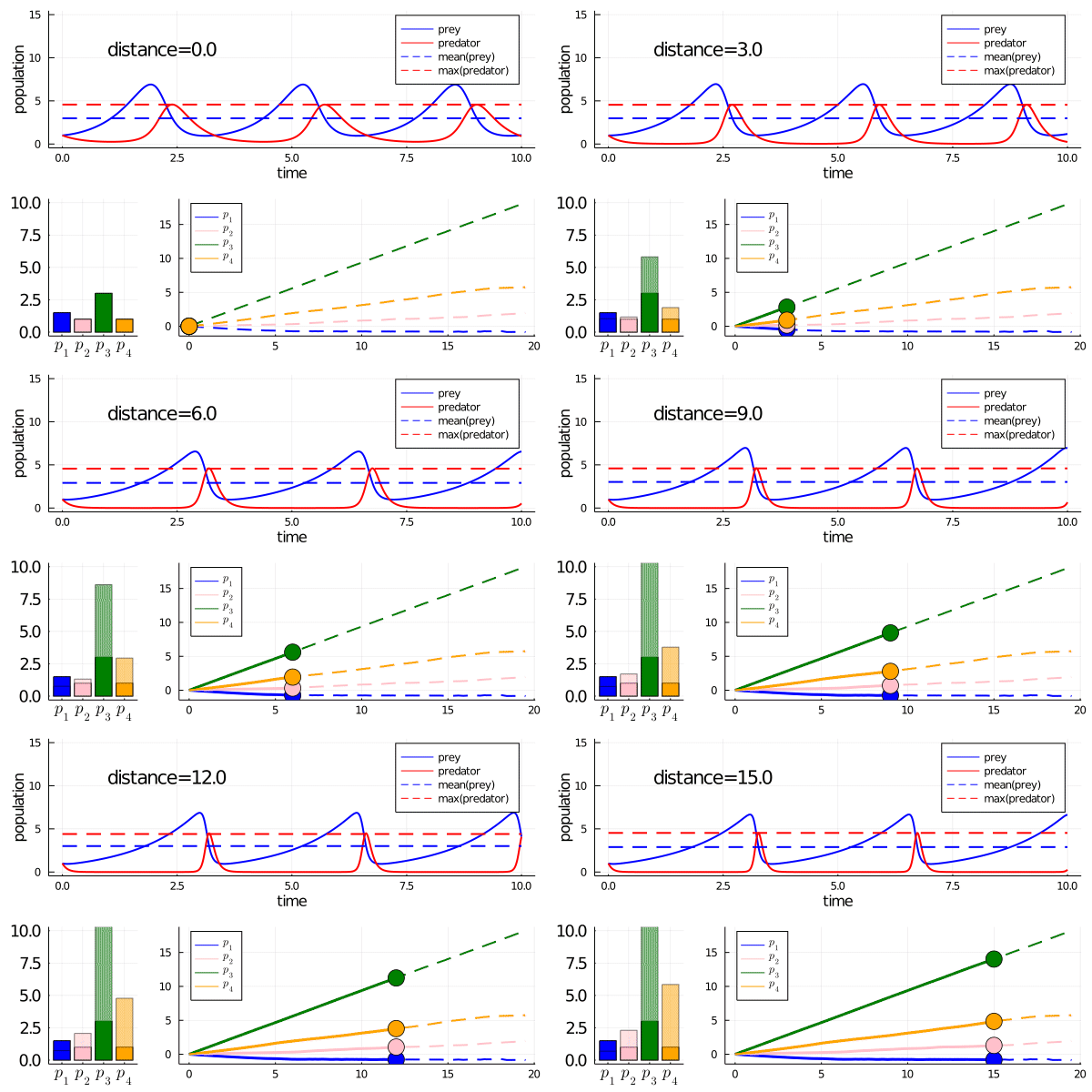
Minimally disruptive curve 1

• As we move along the curve, predators move towards an $r$-strategy, and prey moves towards a $K$-strategy.

• We can also move in the opposite direction (prey to $r$ strategy, predator to $K$). To avoid figure clutter, run the pasted code yourself to see this!

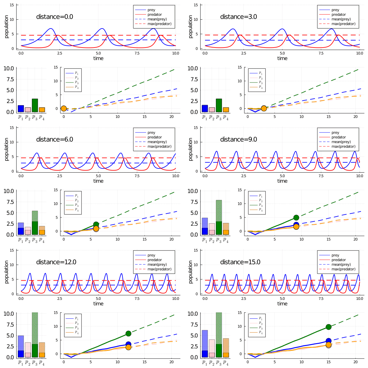
Minimally disruptive curve 2

• This curve instead finds a way to modulate the frequency of predator prey interactions, while preserving model features

• Note how it abruptly changes direction when slowing frequency eventually prevents model features being maintained (as the period approaches the length of simulation). It goes from decreasing the frequency to increasing it.

The code

• Gives static plots of the minimally disruptive curves. Code for the gifs was a bit more involved!

using OrdinaryDiffEq, ForwardDiff, MinimallyDisruptiveCurves, Statistics, Plots, LinearAlgebra, LaTeXStrings

#which md curve to plot
which_dir = 2

## define dynamics of differential equation
function f(du, u, p, t)
    du[1] = p[1] * u[1] - p[2] * u[1] * u[2] #prey
    du[2] = -p[3] * u[2] + p[4] * u[1] * u[2] #predator
end

u0 = [1.0; 1.0] # initial populations
tspan = (0.0, 10.0) #time span to simulate over
t = collect(range(0, stop=10.0, length=200)) # time points to measure
p = [1.5, 1.0, 3.0, 1.0] # initial parameter values
nom_prob = ODEProblem(f, u0, tspan, p) # package as an ODE problem
nom_sol = solve(nom_prob, Tsit5()) # solve 


## Model features of interest are mean prey population, and max predator population (over time)
function features(p)
    prob = remake(nom_prob; p=p)
    sol = solve(prob, Tsit5(); saveat=t)
    return [mean(sol[1, :]), maximum(sol[2, :])]
end

nom_features = features(p)

## loss function, we can take as l2 difference of features vs nominal features
function loss(p)
    prob = remake(nom_prob; p=p)
    p_features = features(p)
    loss = sum(abs2, p_features - nom_features)
    return loss
end

## gradient of loss function
function lossgrad(p, g)
    g[:] = ForwardDiff.gradient(p) do p
        loss(p)
    end
    return loss(p)
end

## package the loss and gradient into a DiffCost structure
cost = DiffCost(loss, lossgrad)

"""
We evaluate the hessian once only, at p.
Why? to find locally insensitive directions of parameter perturbation
The small eigenvalues of the Hessian are one easy way of defining these directions 
"""
hess0 = ForwardDiff.hessian(loss, p)
ev(i) = eigen(hess0).vectors[:, i]

## Now we set up a minimally disruptive curve, with nominal parameters p and initial direction ev(1) 
init_dir = ev(which_dir);
momentum = 1.0;
span = (-15.0, 15.0);
curve_prob = MDCProblem(cost, p, init_dir, momentum, span)
@time mdc = evolve(curve_prob, Tsit5)

function sol_at_p(p)
    prob = remake(nom_prob; p=p)
    sol = solve(prob, Tsit5())
end

p1 = plot(mdc; pnames=[L"p_1" L"p_2" L"p_3" L"p_4"])

cost_vec = [cost(el) for el in eachcol(trajectory(mdc))]
p2 = plot(distances(mdc), log.(cost_vec), ylabel="log(cost)", xlabel="distance", title="cost over MD curve");

mdc_plot = plot(p1, p2, layout=(2, 1), size=(800, 800))

nominal_trajectory = plot(sol_at_p(mdc(0.0)[:states]), label=["prey" "predator"])
perturbed_trajectory = plot(sol_at_p(mdc(-15.0)[:states]), label=["prey" "predator"])

feature_labels = ["mean prey", "max predator"]
for i in 1:2
    hline!(nominal_trajectory, nom_features, linestyle=:dash, label=feature_labels[i])
    hline!(perturbed_trajectory, features(mdc(-15.0)[:states]), linestyle=:dash, label=feature_labels[i])
end

## Different parameters/trajectories at different points on the curve...but features are preserved, i.e. minimally disrupted!
traj_comparison = plot(nominal_trajectory, perturbed_trajectory, layout=(2, 1), xlabel="time", ylabel="population")

Lessons

• MinimallyDisruptiveCurves.jl showed how we could continuously vary the parameters of the Lotka-Volterra model, while preserving

  1. mean prey population over time

  2. max predator population over time

• One strategy (MDC1) was to alter the parameters to increase (decrease) birth and death rates of the predators while decreasing (increasing) those of the prey. Along the axis of $r$-strategies to $K$-strategies, this corresponds to one species moving in one direction, with the other going in reverse.

• Another strategy (MDC2) was to modulate the frequency of the oscillations. MDC2 showed us exactly how to change the parameters to continuously modulate this frequency.